Which AI models can run at the Very Edge?

Artificial Intelligent (AI) has already become pervasive in our everyday life. Nowadays, we are surrounded by numerous intelligent agents that support the human decision process based on real-time data. Typically, our personal data sensed through our own devices, e.g. smartwatches and smartphones, flows to a remote cloud server, where the decision is taken. Hence, the device itself is mostly used for data collection and streaming tasks, which may not be desirable because of privacy and scaling concerns but also energy-efficiency when targeting long battery lifetimes or harvesting solutions.

To address these issues, Greenwaves Technologies is currently aiming at bringing AI agents close to the sensor sources, at the very edge. This solution brings numerous advantages, including the reduced circulation of personal data, and enables intelligence in challenging environments, e.g. for costs or physical reasons. To support the ambitious goal of smart pervasive sensing, the AI community has recently been investigating novel inference Deep Learning (DL) models optimized in terms of the number of parameters, and not only accuracy. But, still, the complexity is too high to run in real-time on current edge platforms. In fact, when leveraging low-power MCUs for smart sensor applications, the size of deployable inference models is limited both from the low memory footprint and the available computational power. Moreover, the limited energy budget poses additional constraints on the architecture of processing units for running complex DL workload on the extreme edge.

We describe here how Greenwaves Technologies covers this gap to bring complex AI agents onto devices at the very edge.

GAP8: A SoC platform tailored for Edge AI

The GAP8 combines several unique features, which match the needs of edge AI applications. Firstly, GAP8 (Figure 1) can be interfaced to a heterogeneous set of external sensors through a smart peripheral sub-system, the Micro-DMA, which autonomously controls the streaming of multiple sensor data. The peripheral region is enriched by a single-core CPU, the Fabric Controller, and a 512kB L2 memory for data buffering. In addition to the Fabric Controller, an 8 core RISC-V parallel compute cluster can be powered-on to accelerate the inference time of AI workloads. The cluster includes a shared instruction cache memory and a 128kB L1 Tightly Coupled Data-Memory (TCDM), working as a scratchpad memory. To boost the energy efficiency, data transfers between L1 and L2 are manually managed through a multi-channel DMA engine. Lastly, the full platform is optimized in terms of power consumption to fit the requirements of battery-powered devices for smart sensing.

If compared to traditional low-power MCUs, GAP8 performs the sensing task with a low-energy budget on the fabric controller side but provides acceleration capabilities for AI tasks thanks to the cluster parallel engine. From a computational viewpoint, deep neural networks are an ‘embarrassingly’ parallel workload that can be efficiently mapped onto the GAP8’s cluster. Along with the HW support, Greenwaves Technologies provides a full SW stack to efficiently map any deep inference model on the GAP8 architecture, as described in the following section.

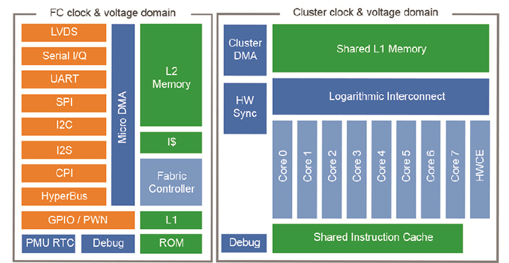
Figure 1 GAP8 Processor Architecture

Deploying a 1000 class Deep Neural Network onto GAP8

To showcase the full process “from a NN framework to GAP8”, this section illustrates the individual building blocks of the Greewaves tool-flow, tailored for the deployment of a deep neural network model on GAP8. To emphasize the GAP8’s capability, we run a MobileNet V1 [1] model trained on a 1000 class image classification problem, which is commonly used also as a backbone network object detection pipelines [2]. The largest model of the MobileNet V1 family, i.e. with an input spatial size of 224×224 and a width multiplier 1.0, features 569 MMAC and 4.2M parameters and reaches a Top1 accuracy of 70.9% on ImageNet. Only by quantizing the parameters to 8 bits, the network can be fully deployed on a GAPUINO system, which couples an 8MB HyperRAM, acting as external L3 memory, together with the GAP8 processor. Details concerning the quantization-aware retraining process are also provided in the next sections.

Basic Computational Kernels

Convolution is the most common operation within a DL workload. Given a convolution layer with an input tensor $a_{i}$ with $I F$ feature channels and a weight tensor $w$ with a receptive field of size $\left(k_{w}, k_{h}\right)$ the output tensor with $O F$ feature channels can be computed by Equation 1 . The result of convolution operation among integer $8 / 16$ -bit operands is scaled with per-layer or per-channel factors $\mathrm{M}$ after the integer feature-wise bias $B$ addition. Such a discretized model derives from [3].

$a_{o}(o f, x, y)=M(o f) \cdot \sum_{i, j, k}^{k_{w}, k_{h}, I F} a_{i}(k, i, j) \cdot w(o f, k, i, j)+B(o f)$

Equation 1 Convolution Layer Integer Model

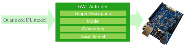
Figure 2 Greenwaves Autotiler Tool

In addition to the 4X/2X memory footprint compression, the quantization of a DL model to 8/16 bit enables the usage of low-bitwidth vector instructions for computing the dot products of Equation 1. In particular, the RISC-V cores of GAP8 come with 2×16 bit and 4x 8-bit SIMD MAC instructions that can be exploited for convolution acceleration. Such optimized instructions are used within a set of software optimized parallel kernels, denoted as Basic Kernels, which implements CNN basic operations and are distributed as part of the GAP8 SDK. These kernels feature low-bit-width operands and assume data residing in shared cluster L1 to gain maximum performance. The functionality of a convolutional network layer can be obtained by grouping together the needed basic kernels. For instance a 3×3 DepthWise layer is composed by KerParConvDWDP3x3Stride1_fps() and KerDPMulBiasScalar_fps() kernels. The first kernel realizes an 8-bit spatial 3×3 depth wise convolution with stride 1 by distributing the workload over multiple cores. The accumulation value, with a bit precision higher than input operands, is scaled by the second call and compressed back to 8 bits.

The GAP Autotiler

Since activation or weight tensors do not typically fit into the L1 memory, an automatic buffering mechanism, denoted as tiling, needs to be implemented by the GAP8 application code. The tiling mechanism transfers data between L3 to L2 and between L2 to L1 memory areas to feed the basic kernel dataflow, and back through the memory hierarchy to store output in memory. To assist programmers, the GAP8 SDK includes the GAP Autotiler tool, that, given the sizes of the convolution layers and the maximum available L1, L2 and L3 memory, automatically determines the optimal tiling strategy. It automatically computes of best size for tensor partitioning, i.e. the tiles of data, that are transferred at any iteration from L2 to L1 and from L3 to L2, and vice versa. The optimal solution is found by minimizing the tiling overhead, measured as the ratio between the total amount of data copied to L1 over the tensor dimension. For any convolution operation, an optimal tiling strategy maximizes data reuse by coping operands to the L1 memory just once, hence the best tiling overhead is equal to 1. It is worth noting that the optimality of the chosen strategy is due to the predictability of the computation dataflow: the GAP Autotiler tool solves the discrete optimization problem by selecting the solution which minimizes the tiling overhead among all the possible solutions.

The GAP Autotiler tool is composed of several building blocks, as depicted in Figure 2. The output of the tool is a C code description of a quantized network graph, which exploits the Basic Kernels mentioned above. The other components will be presented in the next paragraphs, while the quantized input graph can be produced by any DL framework (e.g. Tensorflow or Pytorch).

Generation of Convolutional Network Models

Any DL network can be coded as an Autotiler’s CNN Model, by making use of a set of APIs for the C code generation of CNN layer functions, i.e. the CNN Generators. As an example, the code of the first layer Layer0() of the MobileNetV1 model is generated by calling the Generator:

CNN_ConvolutionMulBiasPoolReLU(“Layer0”, &CtrlH, 1,1,1,1,1,0,0,-7,16,0,1,1,1,0,1,3,32,224,224,KOP_CONV_DP,3,3,1,1,2,2, 1, KOP_NONE, 3,3, 1,1, 2,2, 1, KOP_RELU);

where, besides the convolution parameters, the bit width and quantization of input, weights, output, bias and scaling factor parameters can be individually set. Hence, a GAP Autotiler model can be intuitively described as a sequence of layer generators.

The generator CNN_ConvolutionMulBiasPoolReLU() selects the best basic kernels, determines the tiling strategy and produces the layer C code. The produced code includes the basic kernel calls and the calls to the GAP SDK data transfers APIs that realize the tiling by transferring data from L2 or L3 memory, through generated calls to the DMA and Micro-DMA units. Thanks to this design methodology, the memory management is totally transparent to the user and is overlapped with layer calculation, minimally degrading the performance of the basic kernels.

Graph Generation

The latest release of the GAP8 SDK extends the functionality of the Autotiler tool with a Graph Description input format, aiming at defining the edge connections between the defined nodes, i.e. the layer function generated through the Autotiler’s Generator APIs. Such functionality serves for the generation of the inter-layer glue code to execute the network inference function. The graph is declared and opened by means of the API call CNNGraph_T* CreateGraph (), whose arguments specify the edges of the graph. Nodes are added to the opened graph with the API void AddNode (). For instance, the 21^st layer of MobileNetV1 is appended to the graph by means of:

AddNode(“Layer21”,Bindings(5,GNodeArg(GNA_IN, “OutL20”, 0),GNodeArg(GNA_IN, “FL21”, 0),GNodeArg(GNA_IN, “BL21”, 0),GNodeArg(GNA_IN, “ML21”, 0),GNodeArg(GNA_OUT, “OutL21”, 0) ));

where Layer21 is the name of the generated layer function, while the second argument defines the binding between the edges of the graph and the arguments of the node function created by the layer generator described above. In this case, the 5 arguments of the layer function are connected respectively to OutL20, which is the temporary output of the previous layer, and FL21, BL21 and ML21, are the weight, bias and scaling factor parameters defined during the creation of the graph.

After defining the set of nodes and their connectivity, the call CloseGraph() triggers the processing of the CNN Graph. The output of this process are three C functions, a graph constructor and destructor and a graph runner function for running inference tasks with the given graph.

Figure 3 MobileNetV1 tensor allocation for layer-wise execution with memory constraints of 50kB and 350kB for respectively L1 and L2 buffers

When the graph description is provided to the GAP Autotiler, the memory allocation of both activation and weight tensors, i.e. the edges of the graph, is managed based on the provided memory constraints, i.e. the maximum amount of L1, L2 and L3 memory that can be used. Any activation or parameter tensor is allocated, statically or dynamically depending on the nature of the tensor, on the most convenient memory level and can be promoted at runtime to the L2 memory, if enough memory is available. Figure 3illustrates the allocation of both weight and input activation tensors at runtime when the i-th layer Li of MobileNetV1 is about to be executed. The initial layers, which have a low number of parameters but large input and output feature maps, are mostly kept in L3 while weights are promoted to L2 before layer execution. The opposite strategy is visible on the last layers.

Running the application code

Besides the C-code of the inference function MobileNetCNN(), the GAP Autotiler Tool generates the C-code functions MobileNetCNN_Construct() and MobileNetCNN_Destruct() which, respectively, allocate and deallocate the memory for static parameters. A programmer using the generated code simply calls these in their main application code to run inference tasks on the GAP8 cluster.

Training a Quantized Integer-Only MobileNetV1 model for deployment

Coming back to the input of the Autotiler tool, this section deals with network quantization aspects and targets an audience not familiar with this topic.

To gain maximum performance and the highest compression level, any deep network must be quantized to 8 bits and optionally manipulated to make use only of integer arithmetic. To avoid accuracy loss when using 8-bit quantization, a quantization-aware training process was used. Even for energy and memory-optimized network topologies, such as MobileNet V1 or V2, this has been shown not to reduce accuracy. The quantization strategy we are using symmetrically quantizes the weight parameters around zero, after folding batch normalization parameters inside the convolution layer weights. We use PACT [4] to determine the per-tensor quantization range, however other methodologies can also be applied. The PACT technique is also used to learn the dynamic range of the activation values, i.e. the output of the nonlinear functions.

Given the learned symmetric dynamic range $[-a, a]$ with $a>0$ of any activation or weight tensor, we derive the parameter $S=\frac{2 a}{2^{n}-1},$ based on the number of bits $n,$ as done in [3] Hence, a per-layer scaling factor can be computed as $M=\frac{s_{a_{i}} s_{w}}{s_{a_{o}}}=M_{0} 2^{N_{0}},$ where both $M_{0}$ and $N_{0}$ are parameters quantized to 8 bits.
By definition, $M_{0} \in[0.5,1)$ features a fixed-point $Q 0.7$ format. Given this equation any sub-graph of a fake-quantized model, which starts from the convolution input of the i-th layer and ends with the input of the it1-th convolutional layer, can be approximated with the integer-only Equation 2 without any loss

$a_{o}=\operatorname{clamp}\left(\left(\left(M_{0} \Sigma w \cdot a_{o}+B\right) \gg N_{0}\right), 0,2^{n-1}\right)$

Equation 2 Integer-only approximation of a network sub-graph

of generality. Within the GAP8 toolset, this transfer function is realized by means of combinations of Basic Kernels.
In the case of MobileNet $v 1$ , the described quantization process leads to a final accuracy of $70.03 \%$ on ImageNet, only 0.9\% lower than a full-precision model’.

Experimental Result

Table 1 reports the measurements on GAP8 when running the largest MobileNetV1 network (input resolution 224 and width multiplier 1.0). The network C code is generated automatically by the GAP Autotiler tool, by constraining the usage of L1 and L2 buffer sizes to, respectively, 52kB and 400kB.

Besides the latency and power measurements of the Fabric Controller (FC) region and Cluster (CL), the compute efficiency is reported in terms of MAC/cycles. We benchmarked three configurations, by varying the voltage and frequency settings:

Max Performance: targeting the fastest inference time.
Max Efficiency: maximizing the MAC/cycles metric.
Min Power: targeting the lowest average power consumption.

We show that performance ranges from nearly 2 FPS under a power consumption around 80mW to 0.67 FPS with power consumption as low as 20 mW. Top efficiency of 8 MAC/cycles can be achieved by increasing the memory bandwidth (FC clock).

Table 1 MobileNetV1 224_1.0 running on GAP8

	Max Perf	Max Efficiency	Min Power
CL Freq (MHz)	150	50	50
FC Freq (MHz)	250	250	100
FPS	1.95	0.7	0.67
Vdd (V)	1.2	1.2	1.0
Efficiency (MAC/Clk Cycles)	7.42	8.00	7.64
Avg. Power Consumption CL+FC (mW)	81.2	42	20
Avg Power Consumption IOs (mW)	8.2	3.1	3.4

References

[1] A. G. Howard, M. Zhu, B. Chen, D. Kalenichenko, W. Wang, T. Weyand, M. Andreetto and H. Adam, “MobileNets: Efficient convolutional neural networks for mobile vision applications,” arXiv preprint arXiv:1704.04861, 2017.

[2] W. Liu, D. Anguelov, D. Erhan, C. Szegedy, S. Reed, C.-Y. Fu and A. C. Berg, “SSD: Single shot multibox detector,” in European conference on computer vision, 2016.

[3] B. Jacob, S. Kligys, B. Chen, M. Zhu, M. Tang, A. Howard, H. Adam and D. Kalenichenko, “Quantization and training of neural networks for efficient integer-arithmetic-only inference,” in Proceedings of the IEEE Conference on Computer Vision and Pattern Recognition, 2018.

[4] J. Choi, Z. Wang, S. Venkataramani, P. I.-J. Chuang, V. Srinivasan and K. Gopalakrishnan, “PACT: Parameterized clipping activation for quantized neural networks,” arXiv preprint arXiv:1805.06085, 2018.