

Profiler
A visualization tool for profiling and debugging GAP applications
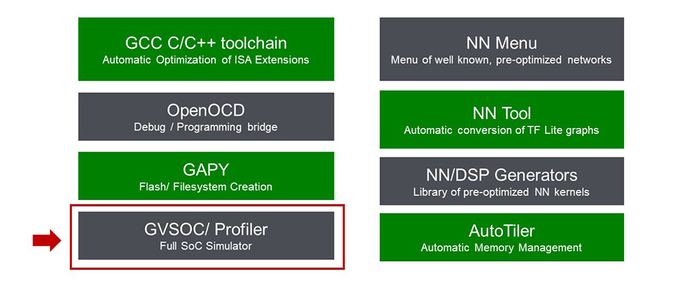
Profiler is a part of our GAP SDK and used with GVSOC, our Full System SoC Simulator. Profiler gives you a visual view of what is happening inside the chip and allows you to control the simulator through a graphic interface. Profiler is an extremely useful tool for developing and debugging applications on GAP processors.
Profiler’s features
● GAP signals display
Profiler displays the internal signals of the GAP processor issued from the GVSOC simulation
● GAP execution overview
Here you can see a chart with the total number of cycles needed by the application on each processing element
● GAP cores traces fine analysis
Here you can view which function is executed at a given timestamp on any core of GAP chip and on the fabric controller
● Stall signals analysis
Here you can view all the stall signals of the GAP cores and fabric controller
● Display of detailed trace Information
Here you can see functions information such as calls number, total execution time, stall signals statistics and source & ASM code in different dock windows
● Display monitoring
With Profiler you can select signals by groups, zooming (button, mouse wheel, double click), time intervals measurement, dock windows management
How to use Profiler to debug the performance of an example application that decodes CIFAR10 images
- Gap SDK and the profiler have been installed. You can now run an example. Let’s go the Cifar10 example directory: cd ~/gap_sdk/examples/autotiler/Cifar10
Now, you can run the profiler with the command “make all profiler platform=gvsoc”
- Profiler launches its main window, which is composed of:
- a central widget called the Timeline window in which all the signals obtained from GVSOC while it runs will be displayed;
- a dock widget that contains a table of all the functions that will be called during the process;
- another dock window that will contain the source code of the function the user wants to examine;
- other dock windows are available and can be selected in the View menu.


- First, you have to define the GVSOC settings and specify which types of signals you want to receive from GVSOC. The Cores and Debug symbols are on by default. Please add the DMAs and stall signals.
- Now please open the signals Tree to select the groups of signals I want to see.
- You can run the CIFAR10 example on the GVSOC platform by clicking on the “Run” button.
- At any moment, you can pause the process by clicking on the “Pause” button. During a pause, a change in the GVSOC settings will have no effect.
- You can also completely stop the process by clicking on the “Stop” button.
- The program can be run again by clicking on the “Run” button with or without changing the settings.
Examining the signals
- Profiler has displayed the selected groups of signals in the Timeline window. The presence of a rectangle on a signal means that the signal has a value of 1. Additionally, the name of the function that is running will be displayed.
- By clicking on a signal rectangle, the line in the Functions table matching the function is highlighted in blue.
- Along with the name of the function, you can see the total time the process spent running this function, the number of calls to the function, and the file containing the source code of the function.
- Additionally, if the source code of the function has been compiled in debug mode, its source code is displayed in the Source Code dock window.
- You can zoom in and out of the Timeline window.
- You can also zoom in and out by using your mouse wheel.

- A scroll bar at the bottom of the timeline allows you to scroll along the whole timeline.
- A “Zoom to fit” button displays the entire timeline.
- Clicking within the Timeline window displays the timestamp pointed by the mouse.
- Clicking and moving the mouse in the Timeline window displays the selected time interval.
Optimizing performance with Profiler on a 3×3 image filter
- The first configuration utilizes just one core in the cluster and loads data from the L2 memory without using the DMA (show code). Thus, we set the number of cores to 1 and DMA to 0.
- We now build and launch the application by running the command “make all profiler=gvsoc.”

- First, we can look at the total time taken by the application, which is roughly 110 ms, spent only on core number 0 and mostly within the call_filter function.
- Now, let us examine the different stall signals for the PE0 core.
- The signal pcer_instr shows the time spent on executing application instructions. We can see that it is not always active and time is lost.
- When pcer_instr is not active, we notice that either the pcer_ld_ext or pcer_st_ext signal is active. These represent the load and store accesses to the external L2 memory.
- We can conclude that the application runs slowly because direct memory access from a cluster core to the L2 memory is slow. The core is not being well utilized. The application is memory bound.

- To avoid those long memory accesses, we will try to load the data from the L2 memory into the shared L1 memory by using a DMA (show code). Thus, we set the DMA to 1.
- We now build the application, launch Profiler, and run the application.
- We can look again at the total time spent by the application, which is now roughly 26 ms, which is much less than when the application was using no DMA.
- Now, let us examine the different stall signals for the PE0 core.
- We now see that the core is executing application instructions on each core cycle.
- In this case, the application runs faster, as there are no more penalties for accessing the L2 memory. The core is now busy; however, the application is now compute bound. Data movement is waiting for the core to complete.


- To avoid the application being compute bound, let us use the 8 cores of the GAP8 processor and parallelize the application. We will now set the number of cores to 8.
- We re-build and re-launch Profiler and run the application.
- We can now see the 8 cores running in parallel.
- Let us examine the total time spent by the application. It is now roughly a bit more than 8 ms.
- In this case, we can see the activity on the 8 cores of the cluster, which results in a performance gain.
- Now, the data movement almost perfectly overlaps with the processing. The application is balanced.
For more information please visit:
| Tools and Software | greenwaves-technologies.com/tools |
| Github project containing the SDK |