Quantization Spec

Quantization of a Neural Network is the process of mapping all the tensors involved in the computation of the graph from their full precision representation (e.g. fp32), into a fixed point representation, with a smaller data type (e.g. int8). This lossy process allows to both reduce the memory requirements of an application (from 32bits to 8bits -> 4x compression) and, in some cases, exploit HW resources to accelerate the operations (like using SIMD instruction or dedicated HW accelerators).

There are many quantization schemes that can be implemented to quantize a neural network (this paper is a good literature review of efficient NN quantization). In this document and our tools we use a similar nomenclature:

Linear (Uniform) Quantization: the quantized values are uniformly spaced in their real representation (can be symmetric or asymmetric)
Non-uniform Quantization: the quantized values are not necessarly uniformly spaced
Floating point: not really a quantization scheme since it uses the floating point representation but still can reduce the memory footprint wrt the full precision model (2x in float16/bfloat16) and still using the floating point arithmetic which adapts the dynamic/precision at runtime.

The schemes above can be implemented in 2 different types of quantization:

Static Quantization: all the inputs of the layer are quantized and the accumulation happens in integer-only arithmetic
Dynamic Quantization: only the constant inputs (weights) of the layer are quantized and the accumulation happens in floating point precision

GAPflow Quantization Schemes and Backend support

Accordingly to the target backend implementation and HW resources, different schemes are supported by the GAP flow:

**Quantization Schemes**
Scheme	Weights Quantization	Activation Quantization	Affine Transformation	Backend support	NNTool Quantization options (passed to G.quantize graph_options or node_options)
POW2	16bit (symmetric, Per-Tensor)	16bit (symmetric, Per-Tensor)	\(r = q * 2^{-N}\)	CHW	Deprecated
Scaled8	8bit (symmetric, Per-Channel)	8bit (symmetric, Per-Tensor)*	\(r = q * S\)	HWC and CHW	hwc=True/False
NE16	2-8bit (symmetric, Per-Channel)	8 or 16bit (asymmetric, Per-Tensor)	\(r = (q - Z) * S\)	HWC	use_ne16=True
Float16	16bit (bfloat16/f16ieee)	16bit (bfloat16/f16ieee)	\(-\)	HWC and CHW	scheme=FLOAT, float_type=float16/bfloat16
Float32	32bit (float32)	32bit (float32)	\(-\)	Only Linear/FC/MatMul/LSTM/GRU/Pooling	scheme=FLOAT, float_type=float32
Float32 Dynamic Quantization	8bit (int8)	32bit (float32)	\(-\)	Only Linear/FC/LSTM/GRU	scheme=FLOAT, float_type=float32, dyn_quantization=True

*: Can be asymmetric if the next layer does not have padding (e.g. padded convolution)

NOTE: Changing quantization type might change the target tensors ordering, for example NE16 conv accelerator works in HWC instead of default CHW. This tensor reordering is done by NNTool automatically after quantization. Hence, the user will need to change the input order accordingly when running inference.

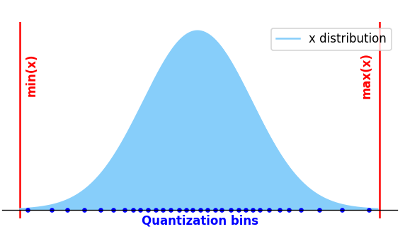
Linear (Uniform) Quantization

The affine transformation that maps real values in uniformly quantized space is the following (quantization function):

\[Q(r) = round(r / S) + Z\]

And the analogous dequantization function is:

\[\hat{r} = S (Q(r) - Z)\]

Where:

\(S = \frac{r_{max} - r_{min}}{2^{nbits}}\): Scaling Factor.
\(Z\): Zero Point, i.e. the quantized (integer domain) representation of the real value 0 (NOTE: the range is constrained, nudged if necessary, to make 0 always representable). This value is always represented in the data type of \(q\). If symmetric quantization, \(Z=0\).

This affine transformation can be applied Per-Tensor (\(S\) and \(Z\) are scalar, one value for every tensor) or Per-Channel (\(S\) and \(Z\) are arrays, one value for every output channel of the weight matrix). Thanks to this representation, the operations of the graph can be moved to integer only arithmetic, leveraging HW acceleration (Conv accelerator, SIMD operations, …). Specifically for symmetric scheme:

\[y = \sum x w \rightarrow S_y Y = \sum S_x X S_w W \rightarrow Y = \frac{S_x S_w}{S_y} \sum X W\]

In this way the \(\sum X W\) is fully integer and can exploit HW acceleration. Once the accumulation is done, the changing scale (from \(S_x*S_w\) to \(S_y\)) is done by an integer multiplication and shift (\(\frac{S_x S_w}{S_y}\) is represented in a fixed point fashion mantissa+exponent, both 8 bits unsigned integers).

In order to quantize the graph, you need to find \(S\) and \(Z\) for every tensor in the graph. To do that, we need to collect statistics of the tensors. NNTool can load this information from the original model (e.g. TFLite or ONNX quantized graph, for example exported from quantization aware training frameworks) or it can run inference in full precision over a calibration dataset and determines the ranges of all the tensors. The collected/loaded tensors ranges might be adapted accordingly to the chosen quantization scheme, e.g. symmetric. This is because our HW might not support directly the scheme loaded from the original tflite/onnx. In the most naive quantization approach, \(S\) and \(Z\) are found using the actual min/max values of the tensors statistics. Other approaches might use different clipping values to avoid including outliers, like \(Mean +/- N*Std\) to take N standard deviations from the tensor mean as min/max values.

\[S = \frac{r_{max} - r_{min}}{2^{nbits}}\]

Future work: Allow the user to pass clipping functions as arguments of the quantization process in order to allow the user to apply any clipping type.

Example

Here is a simple example to quantize the whole graph with static quantization using 5*std values for the weigths and min/max values for the activations, using NE16 backend:

from nntool.api import NNGraph

G = NNGraph.load_graph('mygraph.tflite')
# whatever the original order is, with adjust we move it to CHW
G.adjust_order()
G.fusions("scaled_match_group")

# stats is a dictionary containing for each node the inputs/outputs statistics (std/mean/min/max)
# note that calibration_data_iterator must provide data in the correct order, in this case CHW
stats = G.collect_statistics(calibration_data_iterator())

G.quantize(
   stats,
   schemes=['scaled'],
   graph_options=quantization_options(
     use_ne16=True,
     const_clip_type="std5",
     clip_type="none" #default
   )
)

Non-Uniform Quantization

In this quantization scheme, the quantization steps between consecutive quantized values are not constants:

\[Q(r) = X_{i} \text{ if r} \in [\Delta_{i}, \Delta_{i+1})\]

This scheme typically results in lower quantization noise (because can better represent the statistic distribution) but, since the affine transformation is not linear, it cannot leverage integer-only arithmetic and, therefore, HW acceleration.

In GAPflow this scheme is supported for constants only (weights).

Decompressor

In GAP9+ we support this non-uniform scheme thanks to the decompressor. This HW block allows the data movements between the mem hierarchy using a non-uniform quantization scheme. In particular, the weigths will be stored in their compressed format in L3/L2 and when needed for the computation in L1, the decompressor will extract the values through a programmable LookUp Table. This is typically useful to reduce the precision of floating point constants but still rely in floating point arithmetic (you can save the weights in <8 bits in memory but when the accumulation is computed they will already be in floating point precision, with values extracted by the decompressor in L1).

It can also be used to further quantize uniform quantized values. i.e. the user can uniformly quantize the layer in int8 and further represent the quantized values in int4 (or less) with the decompressor.

Sparsity

Another interesting feature of the decompressor is the sparsity bit. In this mode the decompressor will use a special symbol represented with only 1 bit. This is useful when you have sparse values. It is like a huffman code, where the special value is represented by 1 bit (1’b0) and all the other values are represented by (1b’1 + lut_value). If we have \(N_{items}\) represented with \(Q_b\) bits of which \(N_{spec}\) are mapped to the special value, sparsity is beneficial if:

\[ \begin{align}\begin{aligned}Mem_{non-sparse} = N_{items} * Q_b \text{ [bits]}\\Mem_{sparse} = (N_{items}-N_{spec}) * (Q_b+1) + N_{spec} * 1 \text{ [bits]}\\Mem_{sparse} < Mem_{non-sparse} \text{ if }\\N_{items} < N_{spec} * Q_b\end{aligned}\end{align} \]

Bandwidth implications

An important aspect to take into account when using the decompressor is that, using it, you will reduce the available BW through the L1 from ~8B/cyc to ~2B/Cyc. This is always acceptable if your layer is memory bounded from L3 (the weights loads from L3 is always at ~1B/Cyc so the decompressor will not become a bottleneck). Otherwise, for memory intensive layers (like big linear layers / RNN / etc…), typically memory bounded, you will see the benefits of the decompressor on the execution time only for compression rates >4.

Example

By compressing the weights with non-uniform quantization, NNTool will use KMeans algorithm to find the optimal centroids to represent the weights:

from nntool.api import NNGraph

G = NNGraph.load_graph('mygraph.tflite')
# whatever the original order is, with adjust we move it to CHW
G.adjust_order()
G.fusions("scaled_match_group")

# statistics are not necessarly needed if you want to quantize in floating point
G.quantize(
   schemes=['float'],
   graph_options=quantization_options(
     float_type='bfloat16'
   )
)

# select the constants that you want to compress
const1 = G[1]
# allow_sparse enables the sparsity bit (not always beneficial)
const1.compress_value(bits=6, allow_sparse=False)
# enable/disable compression execution with
G.use_compressed(True)

Floating point

Float16 is a compressed floating point representation (differently from fixed point, dynamic and precision are adapted at runtime). Since it does not have a precomputed \(S\) and \(Z\), tensors statistics is not required. The supported float16 formats in GAP9 are bfloat16 and f16ieee. Also single precision float32 is supported but with limited backend, only Fully connected (Linear) layers, Pooling, MatMul and RNN (GRU/LSTM).

Dynamic Quantization

When using floating point back-end, you can also enable dynamic quantization. This allows you to use compressed weights in 8 bits but the accumulation will be done in floating point:

\[y = \sum x w \rightarrow y = \sum x S_w W \rightarrow y = S_w \sum x W\]

This scheme is useful to get both compression of the weights and full precision for the activations and accumulation.

Limitations: only some layers are supported at the moment (Linear/MatMul/RNN). And only with float32 accumulator/activations.

Example

from nntool.api import NNGraph

G = NNGraph.load_graph('mygraph.tflite')
# whatever the original order is, with adjust we move it to CHW
G.adjust_order()
G.fusions("scaled_match_group")

# statistics are not necessarly needed if you want to quantize in floating point
G.quantize(
   schemes=['float'],
   graph_options=quantization_options(
     float_type='float32',
     dyn_quantization=True
   )
)

Use Case Example

The concepts described above can be applied graph-wise or layer-wise in NNTool, allowing mixed quantization in the whoel graph:

from nntool.api import NNGraph

G = NNGraph.load_graph('mygraph.tflite')
# whatever the original order is, with adjust we move it to CHW
G.adjust_order()
G.fusions("scaled_match_group")

# stats is a dictionary containing for each node the inputs/outputs statistics (std/mean/min/max)
# note that calibration_data_iterator must provide data in the correct order, in this case CHW
stats = G.collect_statistics(calibration_data_iterator())

# select the nodes that you want to port in float / or other schemes
# usually the expression nodes are better in float with no particular impact in the performance
node_opts = {
   node.name:
     quantization_options(
       scheme="float", float_type="float32", hwc=True,
     ) for node in G.nodes(ExpressionFusionNode)
}

G.quantize(
   stats,
   schemes=['scaled'],
   graph_options=quantization_options(
     use_ne16=True,
     const_clip_type="std5",
     clip_type="none" #default
   ),
   node_options=node_opts
)