|
Runtime
Version 1.0
PULP Kernel Library
|
The following command configures the shell environment correctly for the GAP8 SDK. It must be done for each terminal session:
Tip: You can add an "alias" command as following in your .bashrc file:
Typing GAP_SDK will now change to the gap_sdk directory and execute the source command.
This folder contains all the files of the GAP8 SDK, the following table illustrate all the key files and folders:
| Name | Descriptions |
|---|---|
| docs | Runtime API, auto-tiler and example application documentation |
| pulp-os | a simple, PULP Runtime based, open source operating system for GAP8. |
| sourceme.sh | A script for configuring the GAP SDK environment |
| examples | Examples of runtime API usage |
| tools | All the tools necessary for supporting the GAP8 usage |
The hello world example gets each core to print out a hello message. We will go through this example in detail so that you can learn how to schedule tasks on the cluster.
Like other examples and applications, this example is located in the "examples" folder:
Then execute this command for compiling and running the example on GAPUINO:
You can also compile and execute the example separately.
In the result, you will see the Hello from all the cores in FC and in Cluster, with their Cluster IDs and Core IDs.
All the examples can be built and run with the same procedure.
While reviewing this please refer to the runtime API reference.
The hello world main() function is executed on the FC. The runtime uses a simple yet powerful asynchronous event system to synchronize activity between tasks on the FC and the cluster. The first thing the example does is to get a pointer to the default scheduler created when the runtime starts.
You can create more schedulers if your application requires more complex hierarchical scheduling structures.
Each scheduler can queue a certain amount of events. To save memory a fixed amount of space is reserved for queued events. To make sure that we have an adequate amount of queued event space we next add room for 4 queued events.
Now we allocate an event and bind it to a function that will be called when it completes, end_of_call(). We will use this event a little bit later. Note that we bind the CID constant as an argument for the end_of_call function.
Since our hello world example is going to dispatch a task onto the cluster we first need to switch it on. The rt_cluster_mount() call will block until the cluster is switched on when used with a NULL 4th parameter. Many of the asynchronous event based APIs can take NULL as the event argument which transforms them into blocking calls. Whenever blocked the core is clock gated so it consumes minimal power.
Each cluster task is a function called on one of the cluster cores. A cluster function first executes on cluster core 0 which acts as a dispatcher to the other cores. Each cluster core function requires an allocated portion of memory to use as a call stack. We may want to allocate slightly more stack to core 0 to cover the extra tasks associated with dispatching to and collecting results from the other cores. In the case of the hello world example there is not much to do so we allocate the same amount of stack for all the cores.
We allocate the stacks in the cluster level 1 shared memory (RT_ALLOC_CL_DATA) and we get the number of cores in the cluster using rt_nb_pe().
Now we can actually call the function that we want to execute on the cluster using the rt_cluster_call() function. This call will start the function cluster_entry() on core 0 of the cluster and will trigger the event allocated in p_event when the function cluster_entry() exits on core 0. Most APIs that use events can take a NULL pointer for the event parameter. In this case the function will block until completed.
We pass the pointer to the stack area that we have allocated and indicate the size of the stack for core 0 and the size for the other cores and the number of cores that we want to use for this function (all of them).
Just after calling the cluster we trigger events on our scheduler using rt_event_execute(). If no events are ready then this call will block and the core will sleep until one is.
The function cluster_entry() now executes on core 0. We print a message so that you can see the order of execution and start the hello() function on all the cores.
The rt_team_fork() function will block on core 0 until all the cores have exited the hello() function. The hello() function is now executed on all cores including core 0.
Each core in the cluster prints our its core and cluster IDs.
Control now returns to after the rt_team_fork() call which then exits triggering the p_event event on the FC which calls the function end_of_call(). This function executes on the FC and prints out the FC cluster and core IDs. The rt_event_execute() then returns since an event has been serviced. Often we would enclose the call to this function in a loop since we would want to continue waiting for and consuming events but in this simple case we then just turn the cluster off and return terminating the program.
Here is an example of the output:
Notice the control flow, main on FC, then cluster_entry, then hello on all the cores, then return to cluster_entry, then end_of_call and then back to main.
In pulp os, the printf will go through JTAG by default. If you want to console via uart, please define parameter "__rt_iodev" in your program as below:
This global variable will trigger the console on serial port.
As mentioned before, there are three areas of memory in GAP8, the FC L1 memory, the shared L1 cluster memory and the L2 memory. The L2 memory is the home for all code and data. The L1 areas are the location for temporary blocks of data that requires very fast access from the associated core. The shared L1 cluster memory is only accessible when the cluster has been mounted.
All memory allocations are executed by the FC. As opposed to a classic malloc function the amount of memory allocated must be supplied both when allocated and when freed. This reduces the meta data overhead associated with the normal malloc/free logic.
The most portable memory allocator is the one provided by rt_alloc and rt_free.
This takes a first parameter that indicates what the memory is intended to contain. In GAP8 the following areas are used:
| L2 | FC L1 | Cluster L1 |
|---|---|---|
| RT_ALLOC_FC_CODE | RT_ALLOC_FC_DATA | RT_ALLOC_CL_DATA |
| RT_ALLOC_FC_RET_DATA | ||
| RT_ALLOC_CL_CODE | ||
| RT_ALLOC_L2_CL_DATA | ||
| RT_ALLOC_PERIPH |
The asynchronous interactions between the fabric controller, the cluster and the peripherals are managed with events on the fabric controller side.
An event is a function callback which can be pushed to an event scheduler, for a deferred execution. All events in the same scheduler are executed in-order, in a FIFO manner.
In order to manage several levels of event priorities, there may be several event schedulers at the same time. The application is entered with one event scheduler already created in the runtime, which is the one which can be used as the default scheduler. However the application can then create multiple event schedulers in order to build a more complex multi-priority scenario.
Event schedulers are only executed when specific actions are executed by the application. They can be either invoked explicitly by calling rt_event_execute or implicitly when for example no thread is active and the application is blocked waiting for something.
The pool of events which can be pushed to schedulers must be explicitly managed by the application. There is by default no event allocated. They must be first allocated before they can be pushed to schedulers. This allows the application to decide the optimal number of events that it needs depending on the various actions which can occur.
When a scheduler is invoked, it executes all its pending events, unless the current thread is preempted to schedule another thread. To execute an event, it removes it from the queue and executes the associated callback with its argument, until the callback returns. This scheduler can not execute any other event until the callback has returned.
Each thread is assigned an event scheduler. By default, when a thread is created, it is assigned the internal event scheduler. Another scheduler can then be assigned by the application. This scheduler is the one implicitly invoked when the thread is calling a blocking operation such as waiting for an event.
The runtime on the fabric controller is always running a thread scheduler. This scheduler is priority-based and preemptive. Only the ready threads of the highest priority are scheduled following a round-robin policy. It is intended that threads be preempted at a fixed frequency in order to let other threads of the same priority run however this feature is not present in the runtime in the first release of the SDK.
If the application only uses one thread and uses events to schedule tasks (cooperative multi-tasking) it will always run in the main thread. If the application needs to use preemptive threading then it can use the thread API to create new threads. You can find an example of threads and events in the examples/threads_events directory.
The DMA unit that is directly used by the programmer is the cluster-DMA. The micro-DMA is used by peripheral drivers.
The cluster-DMA is used to move data between its 'home location' in L2 memory and the shared L1 cluster memory.
DMA transactions are executed in parallel with code executing on any of the cores. Cluster DMA unit transactions can only be carried out on the cluster. The API should not be used on the FC.
Generally core 0 will be used to set up DMA transfers and then dispatch tasks to the other cores on completion. Each transfer is assigned a transaction identifier. Optionally a new transfer can be merged with a previous one i.e. they shared the same transaction identifier. The rt_dma_wait() function waits until a specific transaction ID has completed.
The DMA queuing function has a 1D and 2D variant. A 1D DMA operation is a classic linear copy. The 2D functions allow a 2D tile where lines have spaces between them to be copied in a single DMA transfer to a continuous memory space.
Take care to declare rt_dma_copy_t copy as a variable and use its address in functions requesting rt_dma_copy_t *copy.
By example, you can find in app_release/examples/dma/test.c:
Since the cluster is viewed as a peripheral to the fabric controller the synchronization model between the two is simple. You start a task on the cluster and it reports a result with an event.
For some algorithms on the cluster you will launch a task on all the cores and each core will carry out the task on its data but may need to synchronize with the other cores at some intermediate step in the operation.
There is a simple scheme to do this using the rt_team_barrier() function. If a cluster core calls this function it will block (clock gated and therefore in a low power state) until all cluster cores in the team have executed rt_team_barrier(). The team is composed of all the cores that were involved in the last rt_team_fork().
You can see this mechanism in operation in the example examples/cluster_sync.
The GAP8 cluster includes a hardware convolution engine which accelerates convolution operations used in CNN. This is not supported in the GVSOC simulator so is not documented in this SDK release.
You can measure performance in two ways, performance counters for cycle level performance and the 32kHz clock for overall execution time.
The cluster and the FC have a range of performance counters that can be used to measure cycle accurate performance on the GVSOC simulator and on the GAP8 hardware.
The following counters are supported on GAP8:
On GAP8 you can monitor RT_PERF_CYCLES and one other event simultaneously on FC and cluster. On the GVSOC simulator it is possible to measure all events simultaneously.
To use the performance counters first initialize an rt_perf_t structure:
Now set the events that you want to monitor:
You can now start and stop the counters around any code that you want to measure.
The counters are cumulative so you can do this multiple times. Whenever you want to get a measurement you call rt_perf_save() and then rt_perf_get() to get individual values:
You can reset the counters at any time with:
Remember that you need to call these functions on the core that you want to monitor.
The 32kHz timer allows you to measure overall execution time. The timer has a resolution of approximately 31us. You can get the value of the 32kHz timer using the function rt_time_get_us().
The HyperBus interface allows external flash and RAM to be connected to GAP. It draws upon the legacy features of both parallel and serial interface memories, while enhancing system performance, ease of design, and system cost reduction. For GAP8 HyperBus, the read throughput is up to 50 MB/s (Max Frequency = 25 MHz).
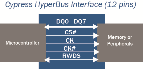
{ width=300px }
For GAP8 HyperBus usage, we recommend implementing HyperFlash and HyperRAM together. For example : GAP8 is connected with S71KS256SC0 [1.8 V, 512 Mbit HyperFlash and 64 Mbit HyperRAM]
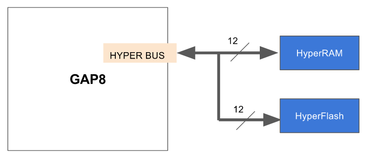
In GAP8 all peripheral access, including HyperBus, is controlled by the micro-DMA unit.
The HyperBus micro-DMA implementation has two channels which both support Flash or RAM. It is normal to configure the two channels as one for Flash and the other for RAM. For example, one for S26KS512S [1.8 V, 512 Mbit (64 Mbyte), HyperFlash™] and the other for S27KS0641 [1.8 V, 128 Mbit (16 Mbyte), HyperRAM™ Self-Refresh DRAM].
In the HyperBus driver, the default channel allocation is channel 0 for HyperRAM and channel 1 for HyperFlash however users can adjust the channel allocation to match their requirements. The driver is responsible for configuring the HyperBus and reading and writing in HyperFlash and HyperRAM. It supports 4 or 2 byte aligned and unaligned access in the following way:
Here are two HyperBus examples, one for HyperRAM and the other for HyperFlash. You can find the examples in the SDK/examples/peripherals/hyper folder.
To indicate to GVSOC that it needs to simulate the HyperRAM, the following line has been added to the Makefile:
read and write functionsrt_hyperram_open opens the correct RAM according to the given device name.rt_hyperram_write writes 1024 bytes from address 0 in HyperRAM. When it finishes, it puts the function end_of_tx in event queue.rt_hyperram_write writes 1024 bytes from address 1024 in HyperRAM. When it finishes, it puts the function end_of_tx in event queue.end_of_tx functions are executed, two read requests read from address 0 and address 1024 separately and will put two functions end_of_rx in event queue.end_of_rx functions are executed then the program exits.To indicate to GVSOC that it needs to simulate the HyperFlash the following line has been added to the Makefile:
read function.rt_flash_open function opens the correct Flash according to device name.rt_flash_read reads 128 bytes from address 0 in HyperFlash, when it finishes, it puts the function end_of_rx in event queue.rt_flash_read reads 128 bytes from address 128 in HyperFlash, when it finishes, it puts the function end_of_rx in event queue.end_of_rx functions are executed, then the program exits.You may want to locate some external files in the HyperFlash simulated by GVSOC so you can use them in a test.
Since the HyperFlash is used by the simulator for the boot code we have provided a read only file system that can be initialized by GVSOC to allow the added files to be read.
The example in the SDK/examples/file_system folder shows how to use the mini file system to locate and read two simulated files.
To use the file system with GVSOC, you need to put this in your makefile:
This will tell GVSOC to load this file into the file system, which can then be mounted, opened, seeked and read by using the file system API.
As the example, you need to use these API as below:
There is an example of using the I2S interface to capture a sound in the directory: SDK/examples/i2s. The example illustrates how to use the I2S driver to connect to digital microphones.
GAP8 embeds 2 I2S modules. Each modules can be connected to 2 microphones so 4 digital microphone can be connected to GAP8. Each modules supports PDM or PCM transfers, sampling frequency initialization, and decimation specification in case of PDM transfer
The following structure is used to configure each I2S module:
By default, this structure is initialized with :
The default settings are:
Initialize an I2S configuration with default values.
Open an I2S device.
Capture a sequence of samples.
Close an opened I2S device.
The example initializes the configuration structure, opens the microphone, and starts the transfer. The transfer is double buffered, optimizing data transfer.
In the folder of examples ($SDK/examples/peripherals/I2S), we provides you a test of a pdm microphones. This test shows you how to use the I2S interface to capture sounds. Thanks to the software model on the platform GVSOC, we can run the microphones without HW.
In this example, a 500Hz sin wave is genarated with sox. The sampling frequency is 44.1kHz. The format of this wave is the standard ".wav". The model of gvsoc will read the stim.wav, and send it to GAP8 via I2S interface. After 1024 samples are received the test will apply a check for verifing the reception is correct.
Be sure that sox and libsndfile are installed :
For testing this example or your application with one microphone on GVSOC platform, please:
At the end of the test, a file storing the received samples is created : samples_waves.hex
You can specify the following options in the CONFIG_OPT variable in the Makefile:
For example :
GAP8 provides a 8 bits parallel interface to connect with an imager, such as HIMAX HM01B0 and Omnivision OV7670. Drivers for these two image sensors have already been implemented in the runtime. There is a high level API in the runtime which abstracts the interface to these cameras.
To use the camera API, the following sequence should be respected:
In the folder of examples (SDK/examples/peripherals/camera_HIMAX), there is an example of using the camera API to capture an image from a Himax imager. Thanks to the emulation in the GVSOC simulator, we can run the camera without hardware.
In this example, the GVSOC reads the file imgTest0.pgm, and sends it to GAP8 via the CPI interface. Once the transfer is finished, the test will apply a check for verifying that the received image is correct. This example takes 2 pictures with different modes:
To test this example or your application with camera on GVSOC platform:
If the image is smaller, the rest of the pixels will be filled by 0xFF. For example, we use an image pgm with size (3 * 3), the image sent by model will be like this:
                                    W=324
    0x55, 0x55, 0x55, 0xFF, 0xFF, 0xFF, ... 0xFF
    0x55, 0x55, 0x55, 0xFF, 0xFF, 0xFF, ... 0xFF
    0x55, 0x55, 0x55, 0xFF, 0xFF, 0xFF, ... 0xFF   H=244
    0xFF, 0xFF, 0xFF, ....                  0xFF
    ............................................
    0xFF....................................0xFF
If you want to use more than 1 image in your application, please name all your image like this: imgTest0.pgm, imgTest1.pgm, imgTest2.pgm ... Then the model will start from the imgTest0.pgm until the last image, and restart from imgTest0.img.
Firstly, please include the runtime header file "rt/rt_api.h", which include sall the libraries in the runtime.
Secondly, please refer to the reference documentation for the GAP8 runtime API.
The Makefile calls the compiler to compile the application with the arguments defined in the Makefile, like how to optimize, which libraries need to be linked, etc.
The name of the final binary can be specified with PULP_APP variable :
The source files that must be compiled to build the binaries can be specified with the PULP_APP_FC_SRCS variable :
The flags (optimize, debug, defines, include paths for examples) that needed to be send to the gcc compiler can be specified with the PULP_CFLAGS variables :
The flags (library paths, libraries for example) that needed to be send to the gcc linker can be specified with the PULP_CFLAGS variables :
The flabs that need to be passed to the gvsoc simulator can be specified with the CONFIG_OPT variable. Some uses of this variable can be seen in the hyperram, cpi, i2s or file system examples :
At the end of your Makefile, please don't forget to add the following include:
Several larger examples are available in the applications directory. These are compiled and run as the other application.
In the first version of the SDK we provide 4 complete applications that highlight examples of various types of image processing:
This section is derived from the GCC documentation.
The first step in using these extensions is to provide the necessary data types. This should be done using an appropriate typedef:
The int type specifies the base type, while the attribute specifies the vector size for the variable, measured in bytes. For example, the declaration above causes the compiler to set the mode for the v4s type to be 4 bytes wide and divided into char sized units. For a 32-bit int this means a vector of 4 units of 1 byte, and the corresponding mode of foo is V4QI in GCC internal parlance.
The vector_size attribute is only applicable to integral and float scalars, although arrays, pointers, and function return values are allowed in conjunction with this construct. Only sizes that are a power of two are currently allowed.
All the basic integer types can be used as base types, both as signed and as unsigned: char, short, int, long, long long. In addition, float and double can be used to build floating-point vector types.
Specifying a combination that is not valid for the current architecture causes GCC to synthesize the instructions using a narrower mode. For example, if you specify a variable of type V4SI and your architecture does not allow for this specific SIMD type, GCC produces code that uses 4 SIs.
The types defined in this manner can be used with a subset of normal C operations. Currently, GCC allows using the following operators on these types: `+, -, *, /, unary minus, ^, |, &, ~, '.
The operations behave like C++ valarrays. Addition is defined as the addition of the corresponding elements of the operands. For example, in the code below, each of the 4 elements in A is added to the corresponding 4 elements in B and the resulting vector is stored in C.
Subtraction, multiplication, division, and the logical operations operate in a similar manner. Likewise, the result of using the unary minus or complement operators on a vector type is a vector whose elements are the negative or complemented values of the corresponding elements in the operand.
It is possible to use shifting operators <<, >> on integer-type vectors. The operation is defined as following: {a0, a1, ..., an} >> {b0, b1, ..., bn} == {a0 >> b0, a1 >> b1, ..., an >> bn}. Vector operands must have the same number of elements.
For convenience, it is allowed to use a binary vector operation where one operand is a scalar. In that case the compiler transforms the scalar operand into a vector where each element is the scalar from the operation. The transformation happens only if the scalar could be safely converted to the vector-element type. Consider the following code.
Vectors can be subscripted as if the vector were an array with the same number of elements and base type. Out of bound accesses invoke undefined behavior at run time. Warnings for out of bound accesses for vector subscription can be enabled with -Warray-bounds. For example you could sum up all the elements of a given vector as shown in the following example:
Vector subscripts are endian independent (GCC code generation generates different code for big and little endian). GAP8 is little endian.
Vector comparison is supported with standard comparison operators: ==, !=, <, <=, >, >=. Comparison operands can be vector expressions of integer-type or real-type. Comparison between integer-type vectors and real-type vectors are not supported. The result of the comparison is a vector of the same width and number of elements as the comparison operands with a signed integral element type.
Vectors are compared element-wise producing 0 when comparison is false and -1 (constant of the appropriate type where all bits are set) otherwise. Consider the following example.
The following example illustrates how to properly compare vectors, in particular how to infer a test that need to be satisfied on a all vector elements and a test that need to be satisfy on at least one vector element.
In C++, the ternary operator ?: is available. a?b:c, where b and c are vectors of the same type and a is an integer vector with the same number of elements of the same size as b and c, computes all three arguments and creates a vector {a[0]?b[0]:c[0], a[1]?b[1]:c[1], ...}. Note that unlike in OpenCL, a is thus interpreted as a != 0 and not a < 0. As in the case of binary operations, this syntax is also accepted when one of b or c is a scalar that is then transformed into a vector. If both b and c are scalars and the type of true?b:c has the same size as the element type of a, then b and c are converted to a vector type whose elements have this type and with the same number of elements as a.
Vector shuffling is available using functions __builtin_shuffle (vec, mask) and __builtin_shuffle (vec0, vec1, mask). Both functions construct a permutation of elements from one or two vectors and return a vector of the same type as the input vector(s). The MASK is an integral vector with the same width (W) and element count (N) as the output vector.
The elements of the input vectors are numbered in memory ordering of VEC0 beginning at 0 and VEC1 beginning at N. The elements of MASK are considered modulo N in the single-operand case and modulo 2*N in the two-operand case.
Consider the following example,
Note that __builtin_shuffle is intentionally semantically compatible with the OpenCL shuffle and shuffle2 functions.
You can declare variables and use them in function calls and returns, as well as in assignments and some casts. You can specify a vector type as a return type for a function. Vector types can also be used as function arguments. It is possible to cast from one vector type to another, provided they are of the same size (in fact, you can also cast vectors to and from other datatypes of the same size).
The previous example is rewritten using a user function to initialize the masks:
You cannot operate between vectors of different lengths or different signedness without a cast.
Even though GAP8 has full support for unaligned accesses GCC will generate better code if you provide an alignment hint:
If you don't, this loop will be vectorized but a complex peeling scheme will be applied ... Performance is reasonable but code size is very bad.
Note also the __restrict__ qualifier, it is essential otherwise you have to assume that a and b can point to the same location making the vector transformation illegal.
Searching a given char (Pat) in a string (A):
Here is another example using plain vectors and bit manipulation function. It returns the index of the first matching instance of Pat in A (compared to a sequential search the execution time is divided by 3). This code will also compile as is on any processor supported by GCC.
Salient features are:
GCC activates auto vectorization when -O3 is passed. You should be aware that at this level of optimization code-bloat might be an issue since loop unrolling, loop peeling and loop realignment lead to a lot of code replication. As a rule of thumb using vector notation as explained in section 3 combined with -O2 is often a better compromise for an embedded target. Beside full target portability is not impacted since these GCC vector extensions are supported on any existing GCC target.
Performing sum of product:
GCC for Gap8 with -O3 will produce the following fully vectorized loop
Performing min/max:
GCC for Gap8 with -O3 will produce the following fully vectorized loop
The last example illustrates the limits of auto vectorization. The following code performs a simple 2D matrix to 2D matrix sum. GCC partially manages to auto vectorize it: the inner loop is fully vectorized but the outer loop is a total mess with lot of code to try to realign the data through partial loop peeling. The exec time will be reasonably acceptable but code-bloat is enormous.
The following code does the same thing but using direct vector notation. SIZE/4 is to account for the fact that a vector contains 4 elements.
Performance is slightly better than auto vectorized version but code size is 10x smaller! Here is code generated for the entire function.
In this section we will illustrate step by step how to optimize a 5 x 5, 2D convolution operating on byte inputs and using byte filter coefficients.
All cycle measurements in these examples were obtained from actual measurements on simulation of GAP8.
We start from a straightforward single core, fixed point implementation in both a basic and then partially unrolled version. Then we use vectorization to improve performance and then further refine the vectorized version. The first step speeds up the code by a factor of 2.84 and the second step by a factor of 2.6. The combination of the two techniques runs with 7.3 times the speed of the straight scalar implementation on one core.
We then show how this single core code is modified to run on the 8 cores of GAP8's cluster, increasing speed by an almost ideal factor of 8. The combination of single core centric optimizations with parallelization leads to an increase in performance of 56.8 times versus the basic single core implementation. It runs in as little as 2.5 processor cycles per full 5 x 5 convolution.
A 5 x 5, 2D convolution is simply a dot product (the sum of the multiplication of each element with the corresponding element) between all the values in the 5 x 5 coefficient matrix and the content of the 5 x 5 square below the coefficient matrix in the input plane.
We obtain all the convolution outputs by sliding the fixed value 5 x 5 coefficient matrix in the 2 directions of the input plane by a step of 1. If the input plane has dimension [WxH] the dimension of the output plane will be [(W-4)x(H-4)].
We assume input data and filter coefficients are fixed point numbers in the [-1.0 .. 1.0] range, in Q7 format[^1]. When two Q7 numbers are multiplied the result is a Q14 number, to normalize it back to Q7 we simply have to shift its content by 7 bits to the right.
A single 5 x 5 convolution output is the result of a sum of 25 products where each product has arguments in the [-1.0 .. 1.0] range, therefore a convolution output is in the [-25.0 .. 25.0] range. In order to avoid overflow we need to right shift the result by 7 + 5, 7 coming from the Q7 format of the inputs and 5 from ceil(log2(25)).
We choose to move down columns first, so we slide the window vertically down the whole height of the input plane before moving to the next vertical strip. This is illustrated in the diagram below:
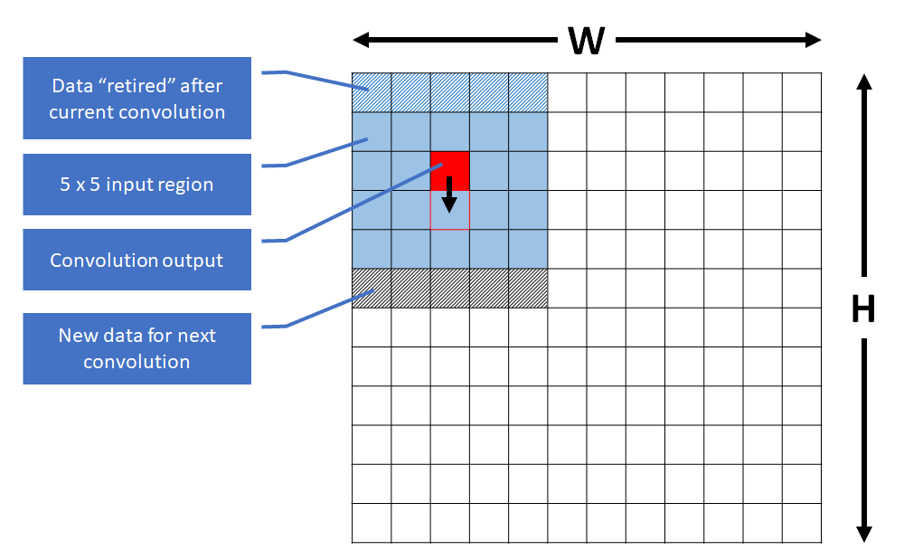
For this first implementation the number of cycles per convolution output is 142.
Below we list the Extended ISA RISC-V assembly code generated by the compiler for the central part of the kernel where most of the complexity is:
Firstly, notice that the compiler has optimized the loops using the GAP8 extended ISA loop setup instructions.
We see that the inner loop is iterated 5 times and at each iteration we do 2 reads and a MAC (multiply/accumulate). Unfortunately the t3 input of the MAC comes from the load in the instruction right before it so we have a 1 cycle stall since the data is not immediately ready. The total impact of this 1 cycle penalty is 25 cycles per convolution output. If we can get rid of this penalty we should be able to get down to 117 cycles per output.
The compiler is pipeline aware and schedules the code in order to minimize stall cycles. Unfortunately in this case the scheduling window is one iteration of the inner loop, there is simply no solution to remove this penalty. One possibility is to try unrolling the loop by compiling in -O2 mode to avoid the code bloating effect coming from systematic in-lining performed with -O3.
Another alternative is to perform partial unrolling of the loop manually. This is what we are going to do in the inner loop:
Running this new code we are now getting 97 cycles per convolution output instead of 142. This is more than expected mostly because the generated code now is also more compact with optimal usage of post modified memory accesses.
If we again dump the generated code we see that the inner loop is now optimally scheduled with no more load use penalty. With this unrolled form we are now very close to the minimum number of instructions needed for a 5 x 5 convolution, 5 * (10 loads + 5 macs) = 75. Here we have 80 (5 x 16) instructions executed:
GAP8 has built-in support for vectors of 4 byte elements or 2 short elements. Among the supported vectorial instructions there is a one cycle dot product. In our case our input data and coefficients are bytes so they are perfect candidates for vectors of 4 elements. A dot product in this configuration computes 4 products and sums them into a 32 bit output optionally accumulating the sum with an existing value in a register in a single cycle.
If V0 and V1 are 2 vectors of 4 bytes each then:
Acc = Acc + V0[0] * V1[0] + V0[1] * V1[1] + V0[2] * V1[2] + V0[3] * V1[3].
Each individual product produces a 32 bit result and this is what makes this instruction extremely interesting because the width of its output is much larger than the width of its inputs avoiding overflow.
The diagram below shows how vectors can be used to compute a given convolution. V0, V1, V2, V3, V4 are vector accesses while B0 to B4 are regular byte accesses:
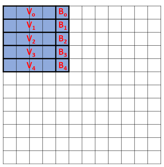
Here is the code that uses this vector layout:
The gap8_sumdotp4() macro expands to the appropriate gcc built-in. Refer to the API documentation for more information.
If we measure the number of cycles obtained with this new code the number of cycles per convolution output is 50.
We could likely save a little bit unrolling the inner loop as in the earlier scalar example however if we look more carefully at this code we can see an even greater optimization possibility by looking at the data that changes between 2 consecutive convolution evaluations.
Obviously the filter stays constant for the entire input plane however 4/5th of the input plane data is also the same between convolution evaluations since we are just sliding the convolution window down by one value. If we can exploit this then we will not only save cycles but also reduce the memory accesses from shared level 1 memory by 80%.
The diagram bellow shows how the vectors are mapped for this strategy and how the vectors are updated when moving from one convolution to the next:
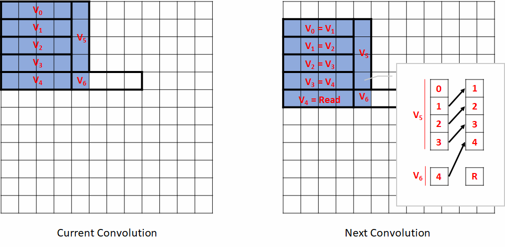
As you can see most of the vectors follow the natural order of the input. V5 is an exception since it is vertical. Only the first element of V6 is used. The right call-out box explains how we build next V6 from current V5 and V6. This process is called vectorial shuffling and is supported by a standard gcc built-in: __builtin_shuffle(V0, V1, ShuffleVector).
In the gcc built-in, the vector's elements are labeled from 0 to N-1 where N is the size of the vector. In our case N=4. ShuffleVector indicates which element to pick from V0 or V1 to produce the ith output. The elements of V0 are numbered from 0 to 3 and V1 from 4 to 7, so for example __builtin_shuffle(V0, V1, (v4s) {7, 0, 1, 5}) will return {V1[3], V0[0], V0[1], V1[1]}. For our case, the permutation vector we need is (v2s) {1, 2, 3, 4}, a simple shift of one value.
Putting everything together we obtain the following code. As you will see there is a bit more going on since we have to take care of priming the vectors at the beginning of each vertical strip in the input data and we also have to use type casts to convert the input data from bytes to vectors:
Here is the generated assembly for this version looking only at what is done for the loop going through an entire vertical strip (for (j=0; j<(H-4); j++) {...}):
As you can see it is extremely compact.
If we measure the number of cycles obtained with this new code the number of cycles per convolution output is 19.
The table below summarizes the cycles per convolution for our 4 versions.
| Algorithm | cycles |
|---|---|
| Initial version | 142 |
| With unrolling | 97 |
| Using vectors | 50 |
| Aggressively using vectors | 19 |
So far we have been using a single core. Now we will see how to modify the code to use all the available cores in the GAP8 cluster.
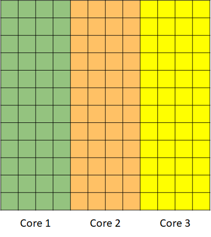
To parallelize the code the most important thing to notice is that the evaluation of one vertical strip is completely independent from the evaluation of the other vertical strips in the input. Given this, it is straightforward to see that if we split the output plane on groups of vertical strips we will be able to provide work to all the cores that are available. The figure below illustrates this. In the diagram below for simplicity we assume we have 3 cores:
The code below shows our initial basic scalar implementation extended to a parallel version:
For all the other code variants the approach is identical.
The table bellow gives the number of cycles per convolution output for our 4 versions, running on 1, 2, 4 and 8 cores.
| 1 core | 2 cores | 4 cores | 8 cores | |
|---|---|---|---|---|
| Initial version | 142 | 71 | 35 | 19 |
| With unrolling | 97.4 | 48.9 | 25.2 | 14.2 |
| Using vectors | 50 | 25.2 | 13 | 7.4 |
| Aggressively using vectors | 19.2 | 9.5 | 4.8 | 2.5 |
You will notice that moving to a parallel implementation has nearly no impact on the performance on 1 core. Also the scaling factor is very close to the ideal as we increase cores, i.e. the cycles decrease proportionally to the number of cores used. In the most aggressive implementation we move from 19.2 down to 2.5 cycles per convolution as we move from 1 to 8 cores, a speed up of a factor 7.68.
If we omit the initial version and compare the result for 1 core with the unrolling version to 8 cores with the most aggressive version we move from 97.4 to 2.5 cycles, an improvement of nearly 39 times.
The way to understand why we are seeing this much improvement is to look at the resources we are using. First we used 4 dimensional vectors, we can expect a 4 times improvement in performance. Next we parallelized the code with 8 cores, another 8 times faster on top of our original 4 times, so 32 times faster in total, consistent with our 39 times observed improvement.
[^1]: See Q fixed point number format - https://en.wikipedia.org/wiki/Q_\(number_format\))

